
Introduction to Support Vector Machines - Motivation and Basics
In this post, you will learn about the basics of Support Vector Machines (SVM), which is a well-regarded supervised machine learning algorithm. This technique needs to be in everyone’s tool-bag especially people who aspire to be a data scientist one day. Since there’s a lot to learn about, I’ll introduce SVM to you across two posts so that you can have a coffee break in between :)
Motivation
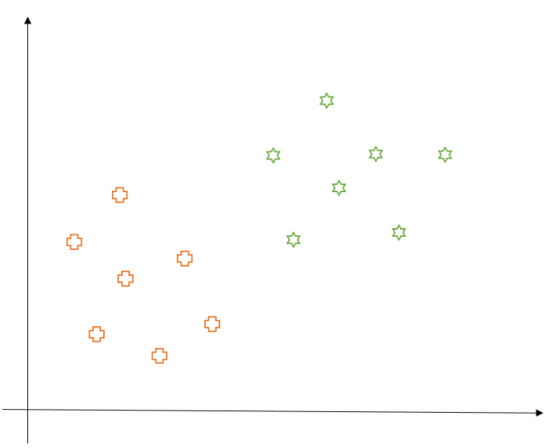
First, let us try to understand the motivation behind SVM in the context of a binary classification problem. In a binary classification problem, our data belong to two classes and we try to find a decision boundary that splits the data into those two classes while making minimum mistakes. Consider the diagram below which represents our (hypothetical) data on a 2-d plane. As we can see, the data is divided into two classes: Pluses and Stars.
Note: For the sake of simplicity, we’ll only consider linearly separable data for now and learn about not linearly separable cases later on.
The goal of SVM, like any classification algorithm, is to find a decision boundary which splits the data into two classes. However, there could be many possible decision boundaries to achieve this purpose like shown below. Which one should we consider?
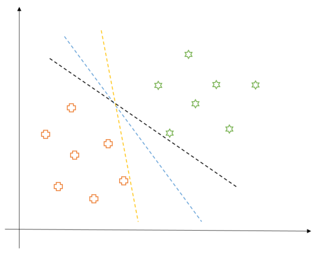
The yellow and the black decision boundaries do not seem to be a good choice. Why, you ask? This is simply because they might not generalize well to new data points as each of them is awfully close to one of the classes. In this sense, the blue line seems to be a good candidate as it is far away from both classes. Hence, by extending this chain of thought, we can say that an ideal decision boundary would be a line that is at a maximum distance from any data point. That is, if we think of the decision boundary as a road, we want that road to be as wide as possible. This is exactly what SVM aims to do.
How it Works (Mathematically)
Now that we understand what SVM aims to do, our next step is to understand how it finds this decision boundary. So, let’s start from scratch with the help of the following diagram.
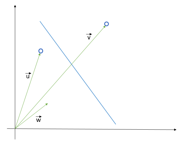
First, we will derive the equation of the decision boundary in terms of the data points. To that end, let us suppose we already have a decision boundary (blue line in above diagram) and two unknown points which we have to classify. We represent these points as vectors $ \vec{u}$ and $ \vec{v}$ in the 2-d space. We also introduce a vector $ \vec{w}$ which we assume is perpendicular to the decision boundary. Now, we project $ \vec{u}$ and $ \vec{v}$ in the direction of $ \vec{w}$ and check whether the projected vector is on the left or right side of the decision boundary based on some threshold $ c$.
Mathematically, we say that a data point $ \vec{x}$ is on the right side of decision boundary (that is, in the Star class) if $ \vec{w} . \vec{x} \ge c$ else it is in the plus class. This means that the equation of the hyperplane (line in case of 2-d) that separates two classes, in terms of an arbitrary data point $ \vec{x}$, is following:
Now we have the equation of our decision boundary but it is not yet immediately clear how it would help us in the maximizing its distance from the data points of both the classes. To that end, we would employ a trick which goes as follows. Usually, in a binary classification problem, the labels of data samples are + 1 or -1. Thus, it would be more convenient for us if our decision rule (i.e. $ \vec{w} . \vec{x} + b$) outputs quantity greater than or equal to +1 for all the data points belonging to star class and quantity less than or equal to -1 for all the data points belonging to plus class.
Mathematically, $ \vec{x}$ should belong to class Star if $ \vec{w} . \vec{x} + b \ge 1$ and $ \vec{x}$ should belong to class Plus if $ \vec{w} . \vec{x} + b \le -1$ or equivalently, we can write
for each point $ \vec{x}_{i}$, where we are considering $ y_{i}$ equal to -1 for plus class and equal to +1 for star class.
These two rules correspond to the dotted lines in the following diagram and the decision boundary is parallel and at equal distance from both. As we can see, the points closest to the decision boundary (on either side) get to dictate its position. Now, since the decision boundary has to be at a maximum distance from the data points, we have to maximize the distance $ d$ between the dotted lines. By the way, these dotted lines are called support vectors.
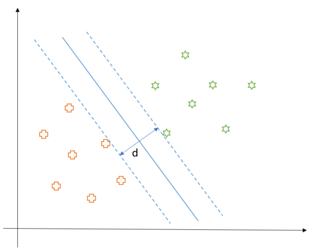
Now, let us denote the closest plus to the decision boundary as $\vec{x}_{-}$ and the closest star as $\vec{x}_{+}$. Then, $d$ is the length of the vector $\vec{x}_{+} - \vec{x}_{-}$ when projected along $\vec{w}$ direction (that is perpendicular to the decision boundary).
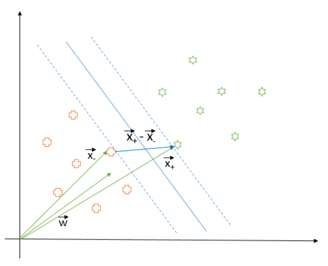
Mathematically, $d$ could be written as:
Since $\vec{x}_{+}$ and $\vec{x}_{-}$ are closest to the decision boundary and touch the dotted lines as mentioned earlier, they satisfy the following equations:
Substituting $\vec{x}_{+}.\vec{w}$ and $\vec{x}_{-}.\vec{w}$ in the equation of d, we get:
Thus, if we have to maximize $d$, we can equivalently minimize $|\vec{w}|$ or minimize $\frac{1}{2} {|\vec{w}|}^{2}$ (this transformation is done for mathematical convenience). However, this optimization must be subjected to a constraint of correctly classifying all the data points. Hence, we’ll make use of Lagrange Multiplier here to enforce the constraint from the equation (A).
Now, it is time to do some mathematics. Formally, our objective is to minimize the following objective function:
Differentiating $L$ with respect to $\vec{w}$, we would obtain the optimal $\vec{w}$ as
The interesting thing to note here is that the decision vector $\vec{w}$ is a linear sum of the input vector (or data points) $\vec{x}_{i}$s. Next step is to differentiate $L$ with respect to $b$ which would give us the following equality
Now, we will substitute (E) into (D) and use (F) to rearrange the objective function into the following:
If you look closely, you would notice that optimization function now depends on the dot product of the input vectors (that is, the data points). This is a nice property to have for the reasons we will discuss later on. Also, this optimization function is convex so we would not get stuck in the local maxima.
Now that we have everything, we could apply optimization routine like gradient descent to find the values of $\lambda$s. I would encourage you to implement it and observe the obtained values of$\lambda$s. Upon observing, you would notice that the value of $\lambda$ would be zero for all the points except the ones which are closest to the decision boundary on the either side. This means that the points which are far away from the decision boundary don’t get a say in deciding where the decision boundary should be. All the importance (through non-zero $\lambda$s) is assigned to the points closest to the boundary, which was our understanding all along.
Does it work on more General Cases?
So, now you know all about what SVM aims at and how it goes about it. But, what about the following case where the data points are not linearly separable:
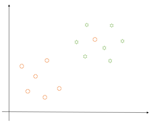
In this case, the SVM would get stuck in finding the optimal position of the decision boundary and we’ll get a poor result at the end of our optimization. Does this mean we can’t apply this technique anymore? The answer is, fortunately, no. For scenarios like these, we have two options:
1 - We can allow our algorithm to make a certain number of mistakes so that other points can still be classified correctly. In this case, we’ll modify our objective function to do just that. This is called the soft margin formulation of SVM.
2 - We can transform our data space into a higher dimension (say from 2d to 3d, but higher dimensions are also possible) in the hope that the points would be linearly separable in that space. We’ll use the “kernel trick” in this case, which would be computationally inexpensive because of the dependence of objective function on the dot product of the input vectors.
Concluding Remarks
We’ll learn about these two methods in the next post. If you have any questions or suggestions, please let me know in the comments. Thanks for reading.