
Text Prediction - Behind the Scenes
These days, one of the common features of a good keyboard application is the prediction of upcoming words. These predictions get better and better as you use the application, thus saving users’ effort. Another application for text prediction is in Search Engines. Predictive search saves effort and guides visitors to results, rather than having them type searches that are slightly off and don’t return a large number of results. As a consumer of these applications, I am sure you would have wondered “How exactly does this prediction works?” at least once. Well, wonder no more because, in this article, I will give you some insight into what goes behind the scenes of producing predictions. So, let’s get started.
Note: This article is going to use some concepts from Probability and Machine Learning theory. I’ll try my best to keep it as general as possible and would provide links to background reading on essential concepts as and when I introduce them.
Predicting text can be thought of as a 3-step process:
Step 1: Representing the problem in terms of a parametric mathematical model.
Step 2: Using historical data to tune the parameters of the model.
Step 3: Making predictions using the tuned mathematical model.
Let’s see what each of these steps entail in detail.
Modeling the problem
This step is also called the Representation step where we represent our knowledge of the problem using a mathematical model. Our goal for this step is to choose a model that accurately captures the relationships between words as they occur in a sentence/paragraph/article. Capturing this relationship would allow us to understand how the occurrences of certain words impact the occurrence of words to follow.
One of the popular class of models for the applications of text prediction is called Markov models of language. The idea of Markov models of language is that the likelihood of occurrence of a word depends on the words preceding it. This is quite understandable as any text has a certain well-defined structure. This structure governs the upcoming words in the text. Mathematically, we can represent this in terms of conditional probability as
One thing to note at this point is that this is a very complex model, as we are considering all the preceding words to define the likelihood of the current word. However, in reality, the occurrence of a word is only impacted by few words preceding it i.e each word is defined by a finite context. Mathematically, this could be represented as:
Here, we are only considering n-1 preceding words to define the likelihood of the $l^{th}$ word. The parameter n controls the model complexity. If n is large, the model would be able to capture intricate relationships between words, but tuning parameters would be computationally expensive. Thus, there is a trade-off in choosing n. The model is called the n-gram model. For this introductory article, we will consider the bigram model (n=2) to make predictions, however, the procedure laid out here would still be applicable to higher order models.
Another simplification we consider for this article would be of position invariance which means that likelihood does not depend on where the words occur in the text as long as their order is same. If V is some vocabulary of words, this can be represented Mathematically as:
Before delving into further details, let me define few terms which I will be using frequently hereafter:
-
Belief Network (BN) - It is a Directed Acyclic Graph (DAG) where each node represents a random variable and each edge represents a conditional dependency.
-
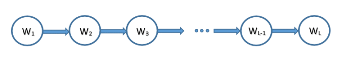
Conditional Probability Table (CPT) - For a node, CPT defines the conditional probability of the node given the state of its parents. We can represent $L$ words bigram model in terms of BN as follows:
CPTs of this model are:
Parameter Tuning
This step is also called the Learning step as we will learn the parameters (CPTs) of the model we introduced in the previous step. To facilitate this, we would collect historical data (or training data) consisting of raw text, which we assume is the natural representation of language’s constructs. This can be done by scraping multiple text-rich websites. Our goal in this step is to learn the parameters that best explain the training data. This is achieved by maximizing the likelihood of occurrence of words in the training data. Mathematically, this means we have to maximize $P(w_1, w_2, …., w_{L})$ where $L$ is the total number of words in the training data.
Now, the goal of maximizing $P(w_1, w_2, …., w_{L})$ is the same as maximizing $log(P(w_1, w_2, …., w_{L}))$. The latter function is called the log-likelihood and will greatly simplify the calculations later on. Thus, we have to maximize:
The relation between the likelihood of the model and the CPTs can easily be found using the product rule as follows:
where $pa(w_l)$ are the parents of $w_l$ in BN.
Let $x$ represent all the values $w_l$ can take, $\pi$ represent all the values $pa(w_l)$ can take and $C_{x\pi}$ represent number of times $w_l$ assumes value $x$ and $pa(w_l)$ assume value $\pi$ together. Then, the likelihood can be written as
Writing log-likelihood in this form would allow CPTs to be optimized independently for each parent configuration $\pi$.
where $\lambda$ is the Lagrange multiplier. We can find optimum for each word (and for each parent configuration $\pi$) by setting the first partial derivative with respect to each word to zero.
Solving the above equation for our bigram model, we would get the following results:
These values of CPTs maximize the likelihood of training data and hence are called the Maximum Likelihood (ML) estimates.
Making Predictions
Our final step is to make predictions using the parameters we learned in the previous step. Suppose, we have already written $l$ words and have to predict the $(l+1)^{th}$ word. The idea is to retrieve all the words that followed the $l^{th}$ word in the training data and select the one having maximum likelihood of occurrence. Mathematically, $(l+1)^{th}$ can be obtained as follows:
From this, we gather that the quality of prediction depends on the training data. If we have a huge amount of data, the counts would tend to be the true representative of the natural occurrence of words. Therefore, the quality of prediction would be good. Keyboard applications/search engines usually learn writing patterns from previous chats/queries and continue doing so as you use the application. That is why the quality of predictions improves with time.
A Toy Problem
Let’s implement the proposed approach on a small dataset (obtained by scrapping several Wall Street Journal articles) to understand it better and to analyze how it behaves.
First, let me provide the description of data files I prepared to perform predictions efficiently. These data files are:
The file vocab.txt contains a list of 500 tokens, corresponding to words, punctuation symbols, and other textual markers. The file unigram.txt contains the counts of each of these tokens in a large text corpus of Wall Street Journal articles. The corpus consisted of roughly 3 million sentences. The file bigram.txt contains the counts of pairs of adjacent words in this same corpus. Let count($w_1$,$w_2$) denote the number of times that word $w_1$ is followed by word $w_2$. The counts are stored in a simple three column format:
One particular thing to note about our initial vocabulary is that there’s an “unknown” token, which represents all the words that occur outside this basic vocabulary. This token is very useful as it is not possible to have all the possible words into our vocabulary, especially in the starting.
Now, let us suppose, we just typed the word THE and want to give top-3 predictions for the next word. Here’s an implementation in python for the same, which I’m going to explain briefly in this article. From step 3, we know that we can obtain the next word using
where $\pi$ would correspond to the token THE in this case. Using vocab.txt, we first obtain the index of THE. Then, we can obtain $C_{\pi}$ from the respective index in unigram.txt. Next, all the words following THE can be obtained from the entries in bigram.txt where the first column has the index of THE. The third column of each of these entries would provide $C_{x\pi}$. Now, we have all the quantities we need to calculate the likelihood of words that follow the token THE. As mentioned in step 2, we can use
to calculate the likelihood. Once we do that, we just have to select top-3 words with highest likelihoods. If we run our implementation of bigram model, top-5 tokens following THE on the basis of likelihood are:
| Token | Likelihood |
|---|---|
<UNK> |
0.615 |
U. |
0.013 |
FIRST |
0.012 |
COMPANY |
0.012 |
NEW |
0.009 |
Having <UNK> as the token with the highest likelihood of occurrence is expected, as most of the words which appear frequently after THE are not in our small vocabulary. This problem can be mitigated with time by augmenting the vocabulary with new words as and when they are encountered. But, until then, we would have to recommend other valid tokens, which in this case are U., FIRST, and COMPANY. This behavior can be linked back to how the keyboard applications behave. Initially, they ask you to give them access to your previous chats to “personalize” the predictions. From there, it builds its initial dictionary. After that, as you use the application, it augments its vocabulary by recording the words you type and improves its quality of prediction.
Concluding Remarks
This brings us to the end of the article about how to predict text using Maximum Likelihood method. Please let me know if you have any queries/feedback in comments. Wishing you a Happy New Year!