
Would this clothing product fit me?
Online shopping is a trend these days as it provides many benefits like convenience, large selection of products, great prices and so on. Trailing on this trend, the online fashion industry has also seen tremendous growth. However, shopping for clothes online is still tricky because it is hard to gauge their fit given the wide size variations across different clothing brands. Thus, automatically providing accurate and personalized fit guidance is critical for improving the online shopping experience and reducing product return rates.
This is an explanatory post of my recent RecSys paper tackling the aforementioned problem. The post is organized as following: Section 1 Formal description of catalog size recommendation problem; Section 2 Brief explanation of a simple machine learning model developed by Amazon last year to tackle this problem; Section 3 Deep dive into the challenges overlooked by the aforementioned model; Section 4 Brief explanation of datasets used to tackle the problem; Section 5 Description of a machine learning model that tries to address those challenges to further improve recommendations; Section 6 Highlights of the results; and Section 7 Open research directions.
Prerequisite concepts
Following concepts are required to understand this post thoroughly. Though I’ll briefly explain some of them, the corresponding links would provide in-depth knowledge.
Catalog Size Recommendation Problem
Many online retailers nowadays allow customers to provide fit feedback (e.g. small, fit or large) on the purchased product size during the product return process or when leaving reviews. For distinction, we will refer to the product (e.g. a Northface Jacket) as parent product and the different size variations (e.g. a Medium sized Northface Jacket) as child products. So, each purchase can be represented as a triple of the form (customer, child product, fit feedback), which contributes two important signals: product size purchased and fit feedback of customer on that size. Given this type of data, the goal of catalog size recommendation is to learn customers’ fit preferences and products’ sizing related properties so that customers can be served with recommendations of better fitting product sizes.
A simple model developed by Amazon
Researchers from Amazon India developed a simple model last year to recommend shoe sizes to customers. For every customer and product, they consider a latent variable which denotes their true size. Let $u_c$ denote the true size for customer $c$ and $v_p$ be the true size for product $p$. They learn these variables using past transactions in which customers have provided their fit feedback. For a product, the true size is different from its catalog size because of the size variations across different brands. The learned true sizes bring the sizing of all the products on the same scale which makes it easier to gauge their fit.
Intuitively, if there’s a transaction ($c$, $p$, fit), then the true sizes $u_c$ and $v_p$ must be close, that is, |$u_c - v_p$| must be small. On the other hand, if there’s a transaction ($c$, $p$, small), then the customer’s true size $u_c$ must be much larger than the product’s true size $v_p$, or equivalently, |$u_c - v_p$| must be large. Similarly, for the large case, $v_p - u_c$ must be large. They assign a fit score to each transaction $t$ as: $f_w(t)=w(u_{t_c} - v_{t_p})$, where $w$ is the non-negative weight parameter, and pose the machine learning objective as: “Given past customer transactions $D$, actual catalog sizes for products, and loss function $L(y_{t} , f_w(t))$ for transactions $t \in D$, compute true sizes {$u_{t_c}$} for customers and {$v_{t_p}$} for child products such that $L = \sum_{t \in D} L(y_t , f_w(t))$ is minimized.”
For the experimentation, they considered Hinge Loss as the loss function. Once true sizes are learned, they use them as features in standard classifiers like Logistic Regression Classifier and Random Forest Classifier to produce the final fit outcome for the recommendation.
Challenges
Although the aforementioned model works, it does not address some key challenges mentioned following:
- Customers’ fit feedback reflects not only the objective match/mismatch between a product’s size and a customer’s measurements but also depends on other subjective characteristics of a product’s style and properties.
- For example, consider a Jacket and a Wet Suit. Usually, customers prefer the fitting of Jacket to be a little bit loose whereas fitting of Wet Suit to be more form fitting. Furthermore, for each customer, fit preferences would also vary across different product categories. Hence, capturing true sizes of customers and products with a single latent variable might not be sufficient.
- Customers’ fit feedback is unevenly distributed as most transactions are reported as
fit, so it is difficult to learn when the purchase would beunfit.- Standard classifiers are not capable of handling the label imbalance issue and results in biased classification, i.e. in this case,
smallandlargeclasses will have poor estimation rate.
- Standard classifiers are not capable of handling the label imbalance issue and results in biased classification, i.e. in this case,
Datasets
Since the dataset used in Amazon’s study was proprietary, for this research we collected datasets from ModCloth and RentTheRunWay websites. These datasets contain self-reported fit feedback from customers as well as other side information like reviews, ratings, product categories, catalog sizes, customers’ measurements, etc. For more details and to access the data, please head over to the dataset page on Kaggle.
A New Approach
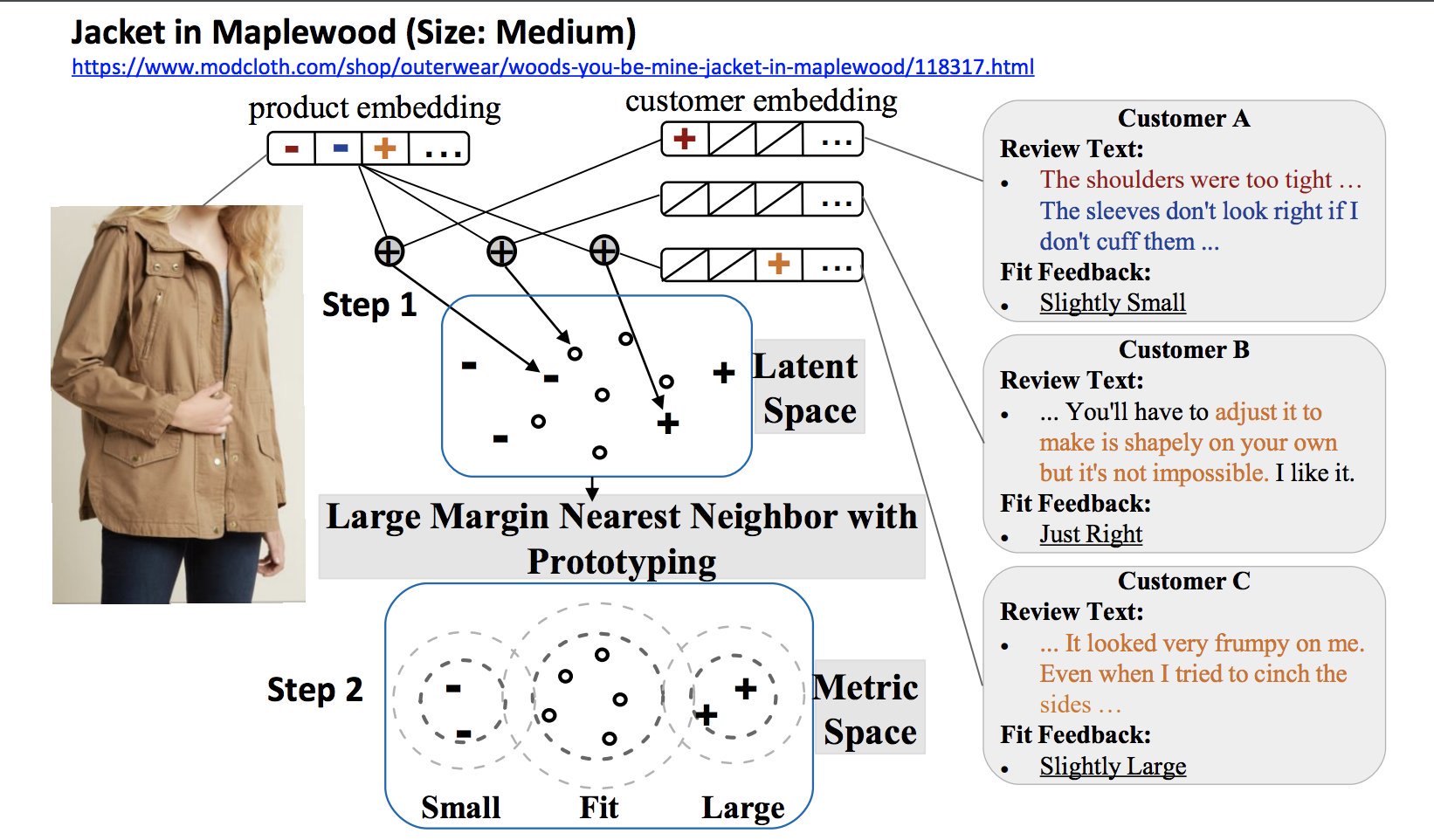
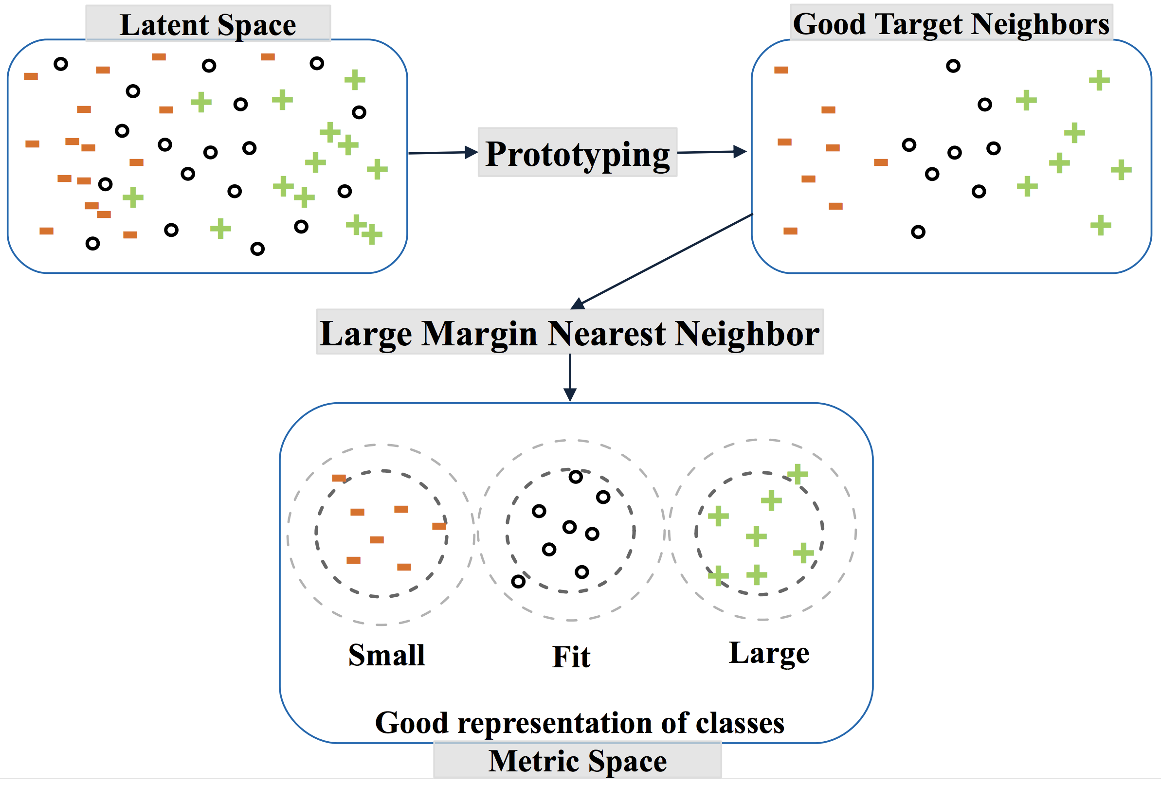
We tackle the aforementioned challenges in the following ways: First, unlike previous work which focuses on recovering “true” sizes, we develop a new model to factorize the semantics of customers’ fit feedback, so that representations can capture customers’ fit preferences on various product aspects (like shoulders, waist, etc.). Second, using a heuristic we sample good representations from each class and project them to a metric space to address label imbalance issues. The overview of the framework can be understood from the following diagram:
We explain our approach in detail in following subsections.
Learning Fit Semantics
Formulation
We quantify the fitness adopting latent factor model formulation as:
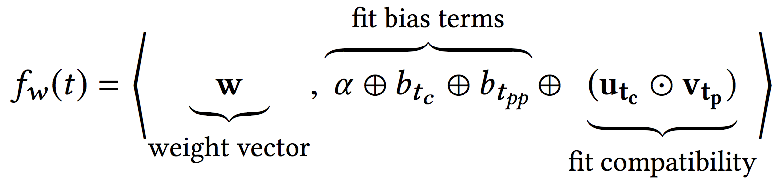
where $\mathbf{u_{t_c}}$ and $\mathbf{v_{t_p}}$ are K-dimensional latent features, $\alpha$ is a global bias term, $\oplus$ denotes concatenation and $\odot$ denotes element-wise product. The bias term $b_{t_{\mathit{pp}}}$ captures the notion that certain parent products tend to be reported more unfit because of their inherent features/build, while $b_{t_c}$ captures the notion that certain customers are highly sensitive to fit while others could be more accommodating.
Furthermore, to enable catalog size recommendation we enforce an order between fitness score of different size variants of a product. This is to ensure that if a product size is small (respectively large) for a customer, all smaller (larger) sizes of the corresponding parent product should also be small (large).
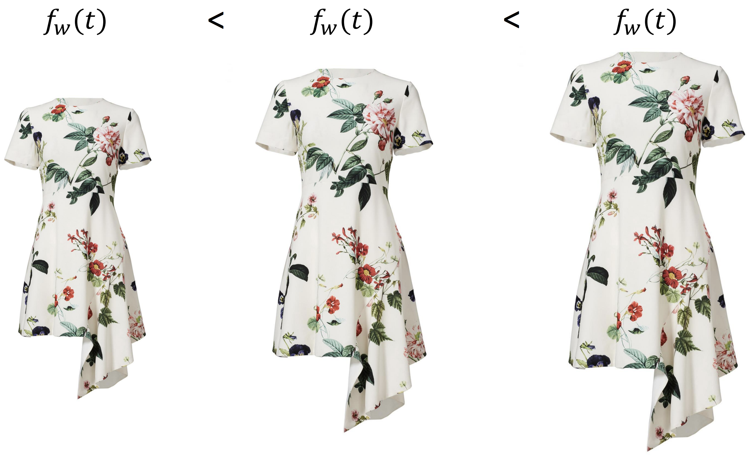
We enforce these constraints by requiring that for each product $p$, all its latent factors are strictly larger (smaller) than the next smaller (larger) catalog product $p^{-}$ ($p^{+}$) if a smaller (larger) size exists. This works since for a given customer ($c$) and parent product ($pp$), fitness scores vary only based on $p$’s parameters.
Optimization
There is an inherent ordering among the output labels small, fit, and large, so it is preferable to model the loss function minimization problem as an ordinal regression problem. We can derive our loss function by reducing the ordinal
regression problem to multiple binary classification problems with the help of threshold parameters.
Let, $b_1$ and $b_2$ are threshold parameters with $b_2 > b_1$ that split the fit score into three segments such that a fit
score greater than $b_2$ corresponds to small, a score less than $b_1$ corresponds to large, and scores in between $b_1$ and $b_2$ correspond to fit. Now, for each of three segments, we can consider greater than threshold score in the positive class and less than threshold score to be in the negative class. Upon solving these three binary classification problems, we can tell which class the purchase transaction belongs to. This concept can be manifested in form of Hinge loss as:
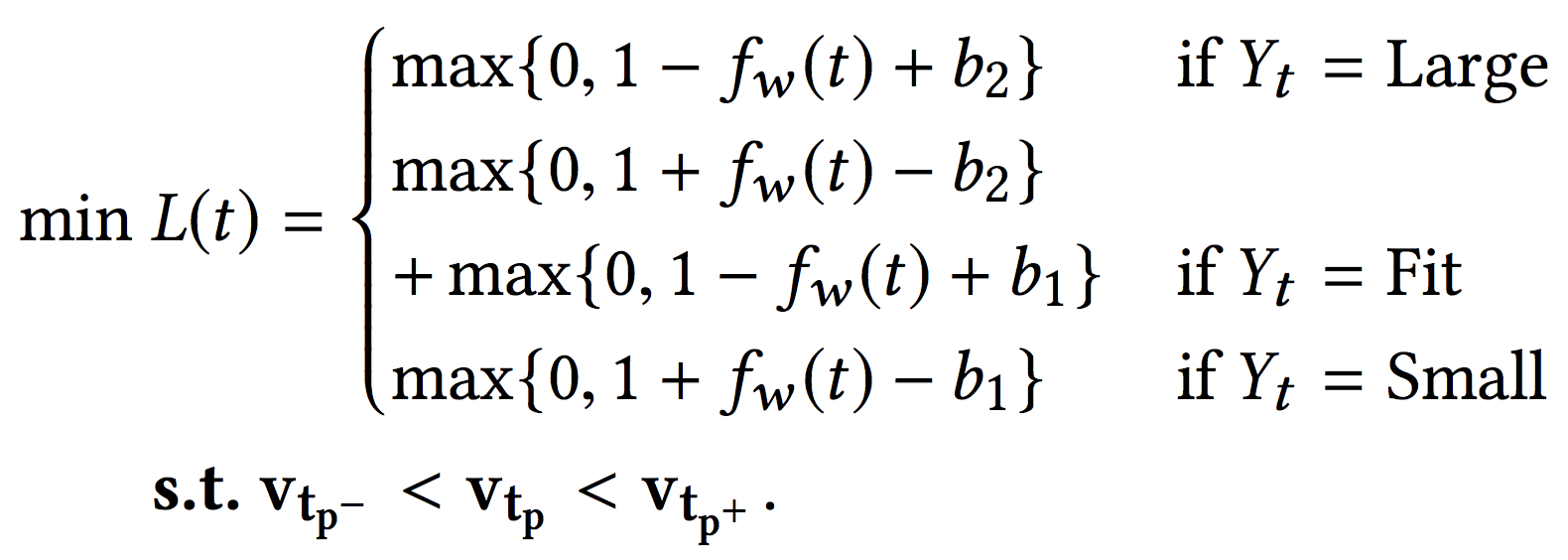
We solve this optimization problem using Projected Gradient Descent method, which is nothing but the Stochastic Gradient Descent procedure with an additional step of enforcing constraints after each update. For monotonicity constraints between $v_{p^{-}}$, $v_{p^{+}}$, and $v_p$, this is as simple as taking the element-wise maximum and minimum.
Handling Label Imbalance
We propose the use of metric learning with prototyping to handle the issue of label imbalance. To that end, our prototyping technique first alters the training data distribution by re-sampling from different classes, which is shown to be effective in handling label imbalance issues. Secondly, we use Large Margin Nearest Neighbor (LMNN) metric learning technique that improves the local data neighborhood by moving transactions having same fit feedback closer and having different fit feedback farther, which is known to improve the overall k-NN classification. This approach is depicted in the following diagram for understandability.
Metric Learning Technique
The goal of metric learning is to learn a distance metric $D$ such that $D(k,l) > D(k,m)$ for any training instance $(k,l,m)$ where transactions $k$ and $l$ are in the same class and $k$ and $m$ are in different classes. In this work, we use an LMNN metric learning approach which, apart from bringing transactions of the same class closer, also aims at maintaining a margin between transactions of different classes. LMNN does this by
- Identifying the target neighbors for each transaction, where target neighbors are those transactions that are desired to be closest to the transaction under consideration (that is, few transactions of the same class)
- Learning a linear transformation of the input space such that the resulting nearest neighbors of a point are indeed its target neighbors. The final classification in LMNN is given by k-NN in a metric space. The distance measure $D$ used by LMNN is the Mahalanobis distance which is parameterized by matrix $L$.
Prototyping
One caveat of LMNN is that it fixes the k target neighbors for each transaction before it runs, which allows constraints to be defined locally. However, this also makes the method very sensitive to the ability of the Euclidean distance to select relevant target neighbors. Prototyping techniques, which aim to select a few representative examples from the data, have been shown to increase processing speed while providing generalizability. Additionally, re-sampling methods are shown to tackle label imbalance issues. Thus, to mitigate the aforementioned limitation of Euclidean distances and tackle label imbalance issues, we develop a heuristic that provides a good representation for each class by reducing noise from outliers and other non-contributing transactions (like the ones which are too close to the centroid of their respective class or to already selected prototypes) by carefully sampling prototypes. You can get more details about the algorithm from the paper.
Experiments and Results
Experimental Setup
We experiment with and compare the following five methods:
- 1-LV-LR: Method proposed in by Amazon as described above. Scoring function is of form $f_w(t)=w(u_{t_c} - v_{t_p})$ and method uses Logistic Regression (LR) for the final classification.
- K-LV-LR: This is a simple extension of 1-LV-LR where $\mathbf{u_{t_c}}$ and $\mathbf{v_{t_p}}$ are $K$ dimensional latent variables.
- K-LF-LR: The proposed latent factor variation given in “Learning Fit Semantics” section. We use the learned factors directly into a Logistic Regression Classifier as features to produce the fit outcome.
- K-LV-ML: This method is similar to K-LV-LR with a difference that it uses Metric Learning, instead of Logistic Regression, to produce the final fit outcome.
- K-LF-ML: This is the proposed method.
These methods are designed to evaluate:
- Effectiveness of capturing fit semantics over “true” sizes
- Importance of learning good latent representations
- Effectiveness of the proposed metric learning approach in handling label imbalance issues.
Results
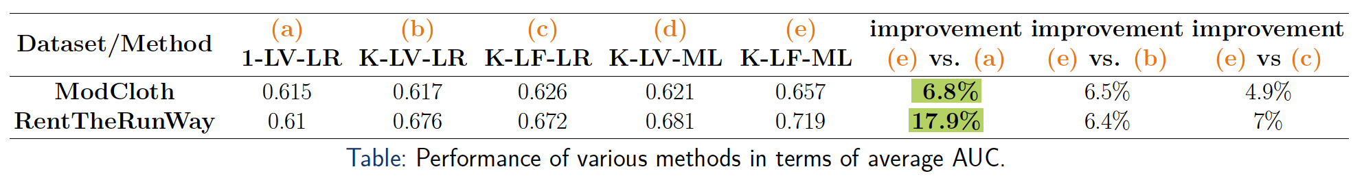
We find that models with $K$-dimensional latent variables outperform the method with one latent variable. Furthermore, we observe that improvements on ModCloth are relatively smaller than improvements on RentTheRunWay. This could be due to ModCloth having relatively more cold products and customers (products and customers with very few transactions) compared to RentTheRunWay (see statistics on dataset page). Of note is that metric learning approaches do not significantly improve performance when using representations from the K-LV method. The reason for this could be that K-LV does not capture biases from data, as bias terms merely act as an extra latent dimension, and learns representations which are not easily separable in the metric space. This underscores the importance of learning good representations for metric learning. Finally, we see that K-LF-ML substantially outperforms all other methods on both datasets.
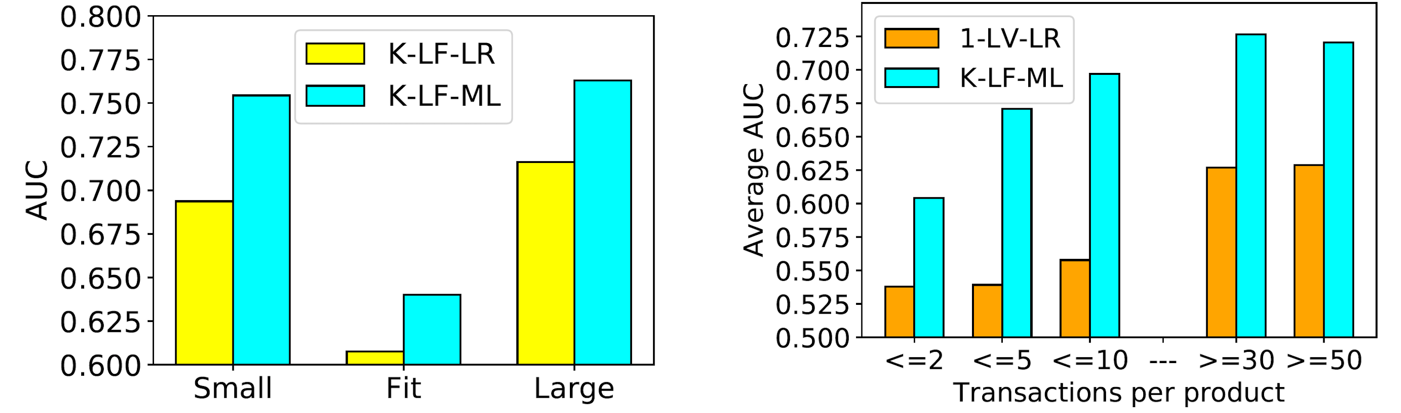
Besides learning good representations, the good performance could be ascribed to the ability of the proposed metric learning approach in handling label imbalance issues as depicted in the above graph. Furthermore, we compare how our method performs in cold-start and warm-start scenarios. For cold products, we notice that K-LF-ML consistently performs better than 1-LV-LR, although their performances are slightly worse overall. As we consider products with more transactions, K-LF-ML improves quickly. The performance of 1-LV-LR improves significantly given sufficiently many samples.
Future Work
One direction for further improvement is utilizing reviews to improve the interpretability of the model since currently, it is hard to understand what each latent dimension correspond to. This is possible by integrating a language model with the latent factor model to assign a specific meaning to each latent dimension (denoted by the corresponding topic) as done in this paper. This would be challenging however, as not all the text mentioned in reviews is relevant to fit and also, many times, customers do not provide fit feedback in detail. Another scope of improvement comes from jointly learning about good prototypes and distance metric as done in this paper.