
Inference using EM algorithm
In the previous post, we learned about scenarios where Expectation Maximization (EM) algorithm could be useful and a basic outline of the algorithm for inferring the model parameters. If you haven’t already, I would encourage you to read that first so that you have the necessary context. In this post, we would dive deeper into understanding the algorithm. First, we would try to understand how EM algorithm optimizes the log-likelihood at every step. Although, a bit mathematical, this would in-turn help us in understanding how we can use various approximation methods for inference when the E-step (calculating posterior of hidden variables given observed variables and parameters) is not tractable. Disclaimer: This post is a bit Mathematical.
Diving Deeper into EM
Let us consider $V$ to be a set of observed variables, $Z$ to be a set of hidden variables and $\theta$ to be a set of parameters. Then, our goal is to find a set of parameters, $\theta$, that maximizes the likelihood of the observed data:
Now, let us consider a distribution $q(Z)$ over the latent variables. For any choice of $q(Z)$, we can decompose the likelihood in the following fashion:
At this point, we should carefully study the form of the above equation. The first term contains joint distribution over $V$ and $Z$ whereas the second term contains conditional distribution of $Z$ given $V$. The second term is a well known distance measure between two distributions and is known as Kullback-Leibler divergence. One of the properties of KL divergence is that it’s always non-negative (i.e $\text{KL}(q||p) \ge 0$). Using this property in (A), we deduce that $\mathcal{L}(q,\theta) \le \text{ln} p(V | \theta)$, that is $\mathcal{L}(q,\theta)$ acts as a lower bound on the log likelihood of data. These observations, very shortly, would help in demostrating that EM algorithm does indeed maximize the log likelihood.
E-step
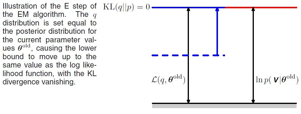
Suppose that the current value of the parameter vector is $\theta^{\text{old}}$. Keeping in mind the relation given by (A), in the E step, we try to maximize the lower bound $\mathcal{L}(q,\theta^{\text{old}})$ with respect to $q(Z)$ while holding $\theta^{\text{old}}$ fixed. The solution to this maximization problem is easily seen by noting that the value of $\text{ln} p(V | \theta^{\text{old}})$ does not depend on $q(Z)$ and so the largest value of $\mathcal{L}(q,\theta^{\text{old}})$ will occur when the Kullback-Leibler divergence vanishes, in other words when $q(Z)$ is equal to the posterior distribution $p(Z | V, \theta^{\text{old}})$. In this case, the lower bound will equal the log likelihood, as illustrated in the following figure [1].
M-step
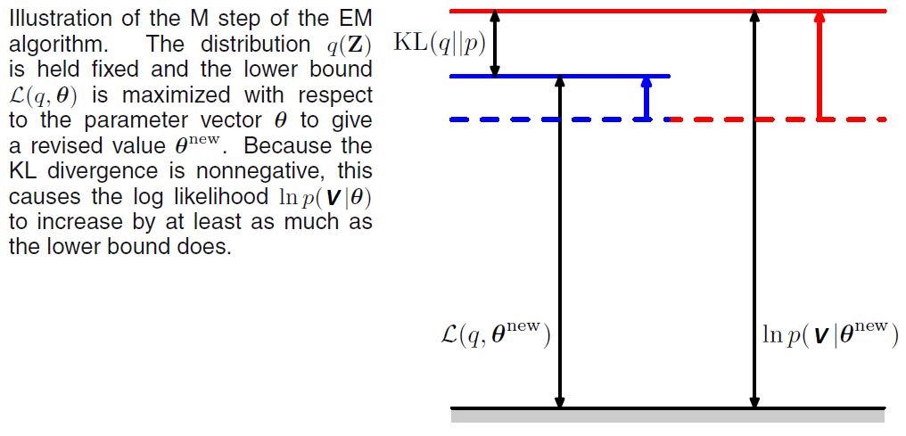
In the subsequent M-step, the distribution $q(Z)$ is held fixed and the lower bound $\mathcal{L}(q,\theta)$ is maximized with respect to $\theta$ to give some new value $\theta^{\text{new}}$. This will cause the lower bound $\mathcal{L}$ to increase (unless it is already at a maximum), which will necessarily cause the corresponding log-likelihood function to increase. Because the distribution $q$ is determined using the old parameter values rather than the new values and is held fixed during the M step, it will not equal the new posterior distribution $p(Z|V, \theta^{\text{new}})$, and hence there will be a nonzero KL divergence. The increase in the log-likelihood function is, therefore, greater than the increase in the lower bound, as shown in the following figure [2].
If we substitute $q(Z) = p(Z|V, \theta^{\text{old}})$ into the expression of $\mathcal{L}$, we see that, after the E step, the lower bound takes the following form:
where the constant is simply the negative entropy of the $q$ distribution and is therefore independent of $\theta$. Thus in the M-step, the quantity that is being maximized is the expectation of the complete-data log likelihood. This is exactly what we saw in the outline of EM algorithm in the previous post.
Putting it all together
I know it’s a lot to digest at once. So, I’ll try to summarize the discussion with the help of following figure [3] which would help in connecting the dots.
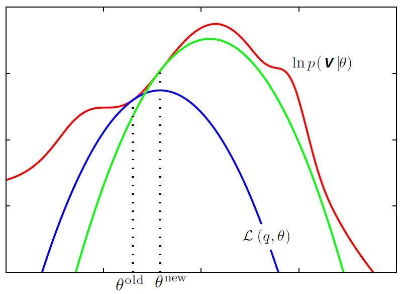
The red curve depicts the in-complete data log likelihood, $\text{ln} p(V | \theta)$, whose value we wish to maximize. We start with some initial parameter value $\theta^{\text{old}}$, and in the first E-step we evaluate the posterior distribution over latent variables, which gives rise to a lower bound $\mathcal{L}(q,\theta^{\text{old}})$ whose value equals the log likelihood at $\theta^{\text{old}}$, as shown by the blue curve. In the M step, the bound is maximized giving the value $\theta^{\text{new}}$, which gives a larger value of log likelihood than $\theta^{\text{old}}$. The subsequent E-step then constructs a bound that is tangential at $\theta^{\text{new}}$ as shown by the green curve.
Approximation methods for inference in EM
As we understood from the previous section, in the EM algorithm, we need to evaluate the expectation of the complete-data log likelihood with respect to the posterior distribution of the latent variables. However, for many models of practical interest, it will be infeasible to evaluate the posterior distribution or indeed to compute expectations with respect to this distribution. This could be because the dimensionality of the latent space is too high to work with directly or because the posterior distribution has a highly complex form for which expectations are not analytically tractable.
In such situations, we need to resort to approximation schemes, and these falls broadly into two classes, according to whether they rely on stochastic or deterministic approximations. Stochastic techniques such as Markov chain Monte Carlo generally have the property that given infinite computational resource, they can generate exact results, and the approximation arises from the use of a finite amount of processor time. On the other hand, we also have deterministic approximation schemes which are based on analytical approximations to the posterior distribution. As such, they can never generate exact results, and so their strengths and weaknesses are complementary to those of sampling methods. One such family of approximation techniques are called variational inference or variational Bayes. Let us try to get some high-level understanding of how each type of technique works.
Markov chain Monte Carlo
Since explaining Markov chain Monte Carlo (MCMC) algorithms in detail is out of scope for this post, I would try to give you a high-level idea about it. MCMC methods comprise a class of algorithms for sampling from a probability distribution. By constructing a Markov chain that has the desired distribution (in this case, the posterior of latent variables) as its equilibrium distribution, one can obtain a sample of the desired distribution by observing the chain after a number of steps. The more steps there are, the more closely the distribution of the sample matches the actual desired distribution.
MCMC could be used to approximate the E Step of EM algorithm for models in which it can’t be performed analytically. So, $\mathcal{Q}(\theta, \theta^{\text{old}})$ from equation (B) could be written as:
where we have used sampling method to obtain $L$ samples, ${Z^{(l)}}$, to approximate the expectation over complete data log likelihood $\mathcal{Q}$. Now, next question you would have in mind is that how do we obtain these samples?
To that end, we would use an MCMC algorithm called Gibbs Sampling. It works as follows: consider the distribution $p(Z | V, \theta^{\text{old}})$ consisting of $M$ hidden variables ${z_1, z_2, …, z_M}$ from which we wish to sample, and suppose that we have chosen some initial values for these variables (could be random). Then, each step of the Gibbs sampling procedure involves replacing the value of one of the variables by a value drawn from the distribution of that variable conditioned on the values of the remaining variables. That is, we replace $z_i$ by a value drawn from the distribution $p(z_i | \{z_{\i}\}, V, \theta^{\text{old}})$, where $z_i$ denotes the $i^{th}$ component of $Z$, and $z_{\i}$ denotes $z_1, … , z_M$ but with $z_i$ omitted. This process is repeated $L$ times to obtain the required samples. Once that is done, the rest of the EM algorithm remains the same. This type of EM algorithm is known as Gibbs EM.
Variational Inference
Unlike MCMC, Variational inference is based on analytical approximations to the posterior distribution, for example by assuming that it factorizes in a particular way or that it has a specific parametric form such as a Gaussian. This type of assumption could also improve the scalability of these methods.
The approximation in Variational Inference comes from considering a restricted family of distributions $q(Z)$ and then seek the member of this family for which the KL divergence is minimized. The goal is to restrict the family sufficiently that they comprise only tractable distributions, while at the same time allowing the family to be sufficiently rich and flexible that it can provide a good approximation to the true posterior distribution.
One such restriction comes from assuming that $q(Z)$ can be factorized as $q(Z) = \Pi_{i=1}^M q_i(Z_i)$ where $Z$ is partitioned into disjoint groups denoted by $Z_i$ where $i= 1, …, M$. Apart from this assumption, we place no restriction on the distributions of individual factors. Without going into Mathematical details, it can be shown that the optimal solution for these factored distributions can be found as:
where
This form of solution conveys that the log of the optimal solution for factor $q_j$ is obtained simply by considering the log of the joint distribution over all hidden and visible variables and then taking the expectation with respect to all of the other factors ${q_i}$ for $i = j$. This and other types of restrictions provide us an easy way to approximate the posterior after which using EM algorithm is straightforward.
Concluding Remarks
This concludes the article. Hopefully, you understood how EM algorithms optimize the log likelihood in each step (E and M) and how we can use some approximation techniques when evaluating the posterior distribution of latent variables is not tractable. Let me know if you have any questions or feedback in the comments. Cheers!