
Maximum Likelihood Estimates - Motivation for EM algorithm
To solve any data science problem, first we obtain a dataset, do exploration on it and then, guided by the findings, we try to come up with a model to tackle the problem. Once all of that is done, our next task is to find a way to estimate the parameters of the model based on the dataset we have, so that we can make predictions on unseen data. In this post, we will learn about how we can learn the parameters of the model using Maximum Likelihood approach which has a very simple premise: find parameters that maximize the likelihood of the observed data. Through that, I would motivate the Expectation-Maximization (EM) algorithm which is considered to be an important tool in statistical analysis. This post would assume familiarity with Logistic Regression.
Maximum Likelihood approach in Logistic Regression
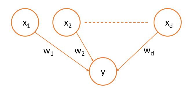
Now, let’s understand the Maximum Likelihood approach in the context of Logistic Regression. Suppose, we have a dataset where we denote predictor variables with $X \in R^d$ and the target variable with $Y \in \{0,1\}$. The model could be depicted graphically as follows:
As we know, prediction probability of target variable in logistic regression is given by a sigmoid function like following:
Based on whether 1 or 0 has more probability of occurring based on the predictor variables, we output our prediction. But, how do we appropriate $w$ such that the error is minimized?
To that end, we will use the Maximum Likelihood approach where we’ll try to find the $w$ which maximizes the likelihood of the observed data. For mathematical convenience, we’ll try to maximize the log of the likelihood. Parameterized by $z$, log likelihood can be written as:
Here the data, $\{x_i,y_i\}^i$ for $i \in {1,2,.., N}$, is represented in terms of multiplication of conditional probabilities $P(Y = y_i | X = x_i)$ with the assumption that data samples are independently and identically distributed (so called the i.i.d assumption). We can expand the equation as:
where we’ve written $P(Y = y_i | X = x_i)$ in a general form such that it is $\sigma(w.x_i)$ when $y_i = 1$ else $\sigma(-w.x_i)$. Upon further simplification, we can write the log likelihood as:
At this point, we should note that log-likelihood $L(w)$ breaks down conveniently into per-instance form. Since there’s no coupling between the parameters, optimization can be done easily and we’ll see later why this is a good thing. Since $L(w)$ is a function of $w$, we don’t have any closed-form solution to equation (A). Thus, we would have to use iterative optimization methods like gradient ascent or Newton’s method to find $w$. An update for the gradient ascent method would look like:
where $\eta$ is an appropriate learning rate. We repeat (B) until convergence. The final value of $w$ we opt for is called maximum likelihood estimate.
Case of latent variables
One detail I didn’t point out about the Logistic Regression model was that all the predictor variables of the model are observed. However, there can be problems that require latent (unobserved) predictor variables in the model. One great example of this kind of model is the Hidden Markov model where the actual state is not directly visible, but the output, dependent on the state, is visible. This model has applications in speech, handwriting, gesture recognition, part-of-speech tagging, musical score following, and other areas. But, does it make any difference in the estimation of parameters if we have hidden variables in our model? Let’s see.
EM algorithm to the Rescue
It turns out, estimating model parameters does get a little tricky if latent variables are involved. Let’s see why. Let $V$ be the observed variables (this includes the target variable) in the model, $Z$ be the latent variables in the model and $\theta$ be the set of model parameters. As per the maximum likelihood approach, our objective to maximize would be:
This can be written in form of conditional probabilities as following:
where $X_j \in \{V_i, Z_i\}$ and $\text{Pa}(X_j)$ represents parent of $X_j$ in belief network of the model. Comparing (A) with (C), we can see that in the latter case, the parameters are coupled with each other because of summation inside the log. Because of this, the optimization using gradient descent or Newton’s method is not straightforward. To estimate the parameters in these situations we use EM algorithm which is composed of two iterative steps both of which try to maximize the objective.
Expectation Maximization (EM) Algorithm
EM algorithm uses the fact that optimization of complete data log likelihood ($P(V,Z|\theta$) is much easier when we know the value of corresponding latent variables (thus, removing the summation from inside of log). However, since the only way to know the value of $Z$ is through posterior $P(Z|V,\theta)$, we instead consider the expected value of complete data log likelihood under the posterior distribution of latent variables. This step of finding the expectation is called the E-step. In the subsequent M-step, we maximize the expectation. Formally, the EM algorithm can be written as:
- Choose initial setting for the parameters $\theta^{\text{old}}$
- E Step Evaluate $P(Z | V, \theta^{\text{old}})$
- M step Evaluate $\theta^{\text{new}}$ given by
- Check for convergence of log likelihood or parameter values. If not converged, then $\theta^{\text{old}} = \theta^{\text{new}}$ and we return to E-step.
Apart from using EM algorithms in models with latent variables, it could also be applied in situations of missing values in data set given that values are missing at random.
Concluding Remarks
This concludes the article. Hope you get a sense of when the EM algorithm proves useful and the high-level idea of how it works. However, as you could guess, usually performing EM steps are not so straightforward. In this follow up post, I expand on the cases where evaluating the posterior (in E step) directly gets intractable and we have to resort to some approximation technique to perform the inference. Let me know if you have any questions or feedback in the comments. Cheers!