
Introduction to Support Vector Machines - Soft Margin Formulation and Kernel Trick
This is the second part of the post on SVM where I’ll discuss Soft Margin Formulation and Kernel trick as ways to tackle linear inseparability problem. First part of the post discusses the motivation and basics of SVM. In the previous part, we left off with the case where the data points did not seem to be linearly separable.
Soft Margin Formulation
Let us discuss our first solution of Soft Margin Formulation, which would allow us to make a few mistakes while keeping the margin as wide as possible.
Motivation
To motivate this technique, please note the following points:
1 - Almost all the real world datasets have data that is not linearly separable. So, we would be presented with cases like these more frequently than we think.
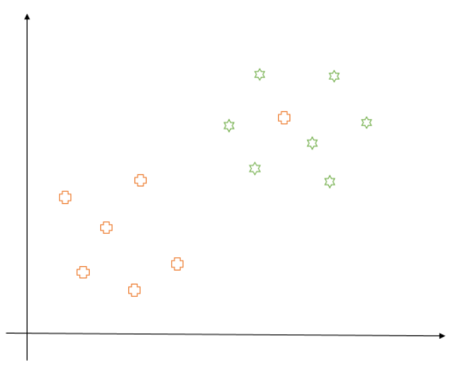
2 - Sometimes, even if the training data is linearly separable, we might not want to choose a decision boundary which perfectly separates the data to avoid overfitting. For example, consider the following diagram:
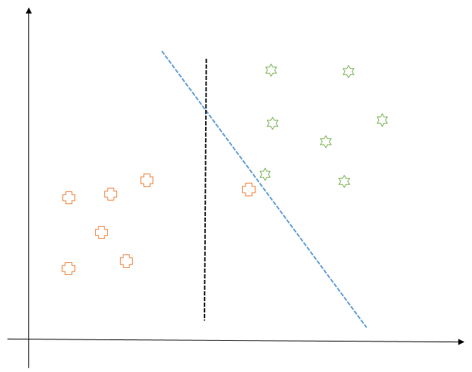
Here, the blue decision boundary perfectly separates all the training points. But is it really recommended to have this line as a decision boundary? Would it be able to generalize well on unseen data? If we think about it, it would not, as it is too close to the points for each class. And for all we know, the plus point close to decision boundary is an outlier or a point labeled incorrectly. Thus, in this case, we would prefer the black line as our decision boundary which makes a minimum number of mistakes while keeping the margin as wide as possible. So, this would be our goal from now on.
How it Works (Mathematically)
Mathematically, our objective should be to minimize
where C is the weight we give to the mistakes. If C is small, it would mean that we give less weight to each mistake and can make a lot of mistakes and if C is large, it would mean we can’t afford to make mistakes and would try to keep it as less as possible. This is a hyper-parameter which we will have to tune by trial and error method.
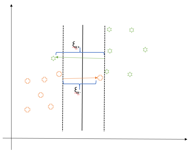
However, all mistakes should not incur the same penalty. Data points on the wrong side of margin which are far away should incur more penalty than the ones close to the margin. Consider the following diagram. We introduce a slack variable $\xi_{i}$ for each data point $x_{i}$ which is nothing but the distance of the point from the margin if it is on the wrong side. So, larger the distance of the point from the margin, more is the penalty. It’s zero for all the points which are classified correctly.
Our objective now is to minimize following:
which loosely translates to maximizing the margin while minimizing the number of mistakes. In this case, our constraint for optimization would also change to following:
The left-hand side of the inequality could be thought of like the confidence of classification. If it is $\ge$ 1, then we are a hundred percent confident that the point is correctly classified and value of the penalty ($\xi$) would be zero. If it is less than 1, we would incur a linear penalty and the value of $\xi$ would be proportional to how far away the point is from the margin.
Next, we’ll make use of Lagrange Multiplier again to enforce the constraint from the equation (B). Formally, our objective would then become to minimize the following with respect to $\vec{w}, b, \xi_{i}$:
Subsequently, we have to follow the same process we followed in the first part of the post. We first do partial differentiation with respect to the variables we want to optimize, then replace the obtained value in our objective function and optimize to find the values of $\lambda$s. In this case, our $\lambda$s would non-zero for the points which are closest to the margin as well as the points which are on the wrong side of the margin. This is because they’ll play a key role in deciding the position of the decision boundary. Thus, these points would constitute our support vectors in the case of Soft Margin formulation.
Kernel Trick
Now, let us explore the second solution of using “Kernel trick” to tackle the problem of linear inseparability. Kernel functions are generalized functions which could be thought of as a black box which takes two vectors (of any dimension) as input and output how similar they are. Some popular kernel functions used in SVM could be found here.
Motivation
Just as a recap, the objective function from the previous part is as follows:
Here we observed its dependence on dot product between input vector pairs. This dot product is nothing but the similarity measure between the two vectors. If the dot product is a small quantity, we say the vectors are very different and if it is large, we say they are quite similar. Hence, in order to generalize our objective function to higher dimensional spaces (and thus posing the problem of separating data points in multidimensional space), we can replace this dot product with the kernel function.
How it Works (Mathematically)
Mathematically, a kernel function can be written as:
Here $x$ and $y$ are input vectors and $\phi$ is a transformation function. Thus, kernel function essentially takes the dot product of transformed input vectors.
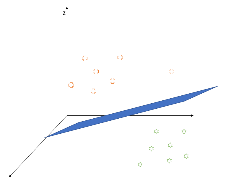
Now, the trick to tackle linear separability problem in two-dimensional space is to project/transform the input vectors into higher dimensional space and hope that the data points now can be perfectly separable by a hyperplane in that space like shown in the figure below.
These transformations are computationally expensive except for the cases where the objective function (which we care to optimize) depends on the dot product of the input vectors. This is perfect for us! The reason behind this exception is that the dot product of the transformed vectors (that is the kernel function) turns out to be a simple function of the dot product of the original vectors. In other words, a simple transformation of the dot product of input vectors could tell us the similarity between them in a higher dimensional space. Pretty great, right?!
Let us take a simple example to give you a better understanding of this technique. Suppose we have the following linearly inseparable data. Clearly, soft margin formulation won’t work well here as any linear decision boundary would make a lot of mistakes. Instead, let us try to apply kernel trick to map this 2-dimensional data to 3 dimensions.
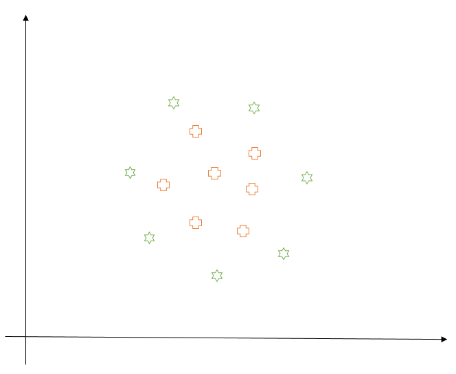
Let us take two points $P_1 = (x_{1}, y_{1})$ and $P_2 = (x_{2}, y_{2})$, and define a transformation $\phi(x,y) = (x^{2},y^{2}, \sqrt{2}xy)$. So, the kernel function (or the similarity function) between any two points can be defined as:
If you observe, the right-hand side of the equation is an equation of a circle in 2-dimensional space. Thus, our notion of similarity is now changed. Instead of saying points on the same side of the line are similar, we say points which together fall inside or outside a circle are similar. In this sense, this trick lets us have a non-linear decision boundary in 2-d space.
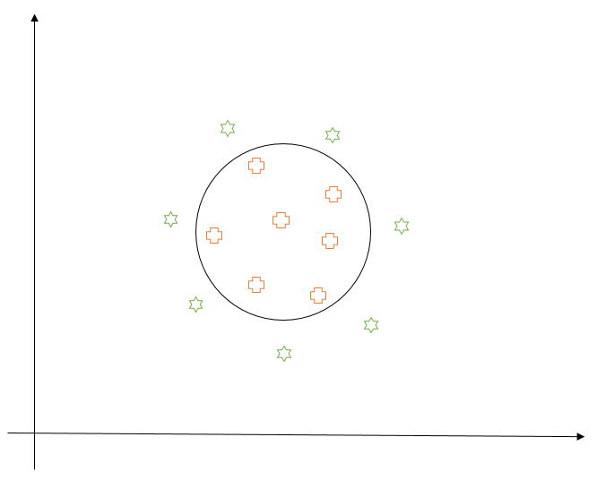
When we project these points into 3-dimensional space, points near the origin of the circle (that is pluses) would move upward (along the z-axis) less than the points far away from the origin (the stars). So, we can easily find a hyperplane which would separate the two classes in 3-dimensional space. This video provides a good visualization of the same.
But, how’s the transformation inexpensive, you ask? Let us further simplify the kernel function:
Hence, as we see, the kernel function is nothing but a simple transformation of the dot product of input vectors, making this technique computationally inexpensive. We usually choose the appropriate kernel function for our application based on our domain knowledge and by cross-validating.
Concluding Remarks
With this, we reached the end of this post. Hopefully, the details I provided here helped you in some way in understanding SVM more clearly. In case you have any questions or suggestions, please let me know in comments. Cheers!